Configuring a fine-tune run
Walk through every leg of the Action Module: base model, dataset, training config, LoRA config, plus the defaults that work for most first runs.
A Fine-Tune Action Module on the Studio canvas has four required legs: base model, dataset, training config, and LoRA config. Once all four are connected, the play button activates and you can queue the run. There is also an optional fifth leg, the Inference node, which sets the sampling defaults baked into the exported model; leave it off and the run uses sensible defaults. This page walks through each leg, including the defaults Ertas uses and when you might want to change them.
If you have not picked a base model yet, start with Picking a base model. For dataset prep, see the Datasets section.
Add a Fine-Tune Action Module
From the canvas in Build mode:
Open the Action Module picker
Click the action picker in the bottom toolbar and choose Fine-Tune. Studio drops a new module on the canvas. Each module has four hanging dashed lines: red for Base Model, blue for Training Dataset, purple for Training Config, teal for LoRA Config.
Rename and describe the recipe (optional)
Hover the module and click the pencil icon. Give the run a name like "Support v3, larger LR" so it is recognisable in the Run panel later. The description is optional, but a one-line "why am I trying this" pays off when you revisit a project months later.
The Fine-Tune module also has Duplicate (purple) and Play (green) icons that appear on hover. Duplicate copies the entire recipe including child nodes; Play queues the run.
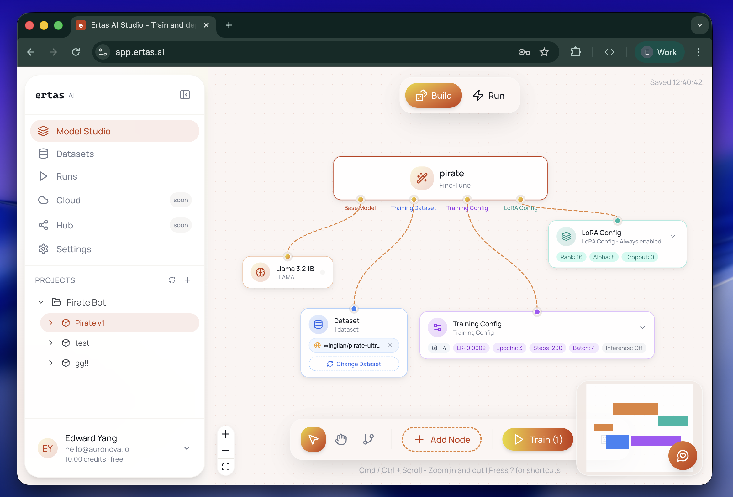
Attach a base model
Click the + under the red Base Model leg. The model picker opens. See Picking a base model for the full decision guide.
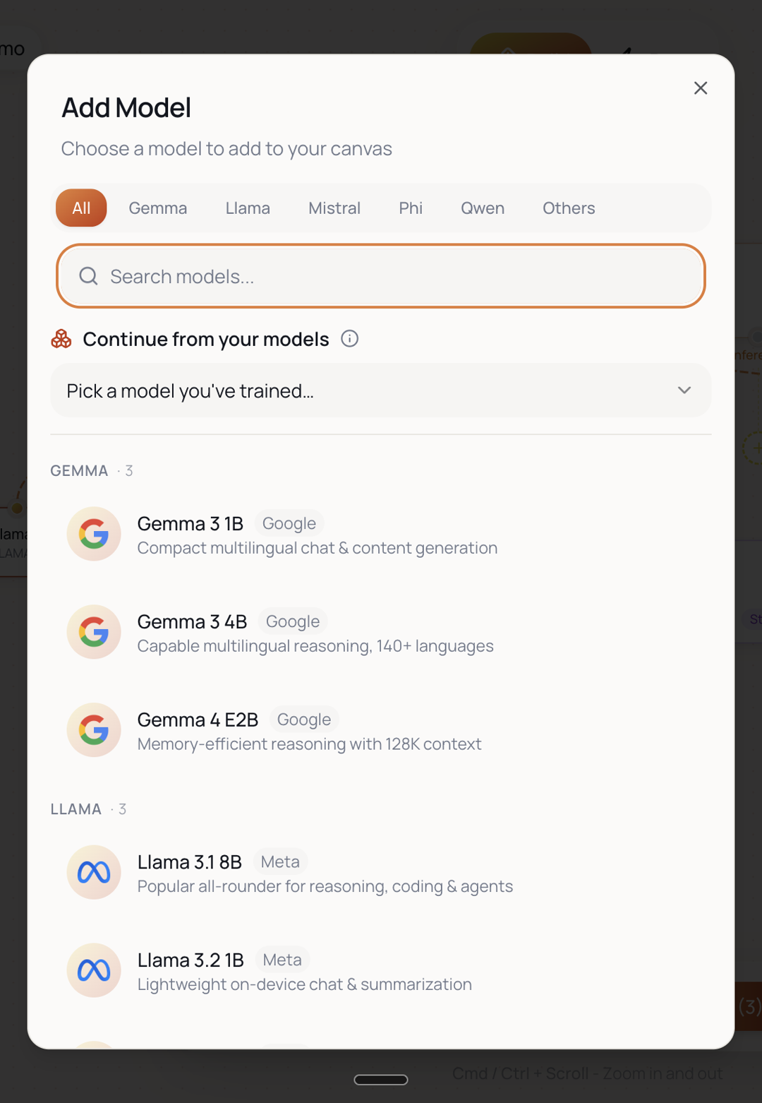
Once a model is attached, the leg goes green and the model node shows the family icon, the model name, and the model type (Llama, Mistral, HF, etc.). Hovering the model node surfaces a Change pill that opens the picker again without disconnecting the leg.
If you change the base model after configuring the Training Config, Ertas normalises the GPU tier upward if the new model requires it. You will see the GPU dropdown auto-update the next time you open the Training Config picker.
Attach a dataset
Click the + under the blue Training Dataset leg. The dataset picker shows three groups:
- Recommended: a small list of curated Hugging Face datasets that are great for first-time fine-tunes (Alpaca Cleaned, Pirate UltraChat, and friends). One click attaches them after a quick validation.
- HuggingFace: datasets you have previously imported from Hugging Face.
- Uploaded: JSONL, CSV, parquet, or txt files you have uploaded yourself.
You can also paste a Hugging Face dataset URL directly. Ertas validates the dataset:
- Confirms it has training-friendly columns (instruction / output, or messages, or prompt / completion).
- Reports row count, file size, and the detected format.
- Asks you to attest you have the right to use the data before saving it to Data Craft.
After attachment, the dataset node shows the dataset name, format, row count, and size. See JSONL format for the exact schemas.
You can attach multiple datasets to a single run by selecting more than one in the picker. Ertas concatenates and shuffles them at training time. Mixing formats (instruction + conversations) is allowed and Ertas handles the templating per row.
Set up the Training Config
Click the + under the purple Training Config leg. The Training Config picker controls hyperparameters and the GPU.
The defaults are tuned to be the fastest path to a useful first run on a 3B to 8B model:
| Field | Default | When to change it |
|---|---|---|
| GPU | T4 (16 GB) | Switch to A10G for models above 8B, longer contexts, or larger batches. |
| Max Steps | 200 | Bump for larger datasets (rule of thumb: 1 step per 8 rows). Set to 0 to use Epochs instead. |
| Learning Rate | 2e-4 | Lower (1e-4) for delicate behaviour tuning; higher (3e-4) for stylistic transfer on small datasets. |
| Batch Size | 2 | Increase if VRAM allows (A10G can usually handle 4 or 8). |
| Epochs | 3 | Only used when Max Steps is 0. |
| Warmup Steps | 15 | Keep at roughly 7% of total steps. |
| Gradient Accumulation Steps | 4 | Combined with batch size, gives an effective batch size of 8. |
| Optimizer | AdamW | Adafactor saves memory at a small quality cost. SGD is for advanced experiments. |
| Convert to GGUF | On | Turn off if you only want the raw LoRA adapter (saves about 12 minutes). |
The "Max Steps vs Epochs" toggle is one of the more common sources of confusion:
- Max Steps > 0: the run trains for exactly that many gradient steps, regardless of dataset size. Predictable runtime and cost.
- Max Steps = 0: the run walks the dataset for the configured Epochs. Total step count is
(rows / effective_batch_size) * epochs.
Pick step-based training when you are iterating on hyperparameters and want apples-to-apples runtime. Pick epoch-based when you have a fixed dataset and want a fixed amount of exposure per row.
GGUF conversion toggle
Convert to GGUF is on by default. It produces a Q4_K_M quantised model at the end of training. Turning it off makes the run finish about 12 minutes earlier and saves a small amount of credits, but you only get the raw LoRA adapter as the artifact. Useful when:
- You want to merge the adapter into a different base in your own code.
- You want to test the LoRA before paying for the quantization step.
You can always rerun a completed job with GGUF conversion enabled if you decide later you want the export.
Attach an Inference node (optional)
Temperature and Top P used to sit at the bottom of the Training Config picker. They now live on their own Inference node, attached to the Action Module's inference leg, so the settings that describe how the finished model generates are separate from the settings that describe how it trains.
| Field | Default | What it does |
|---|---|---|
| Temperature | 0.7 | Sampling temperature baked into the bundled Ollama Modelfile. |
| Top P | 0.9 | Nucleus sampling cutoff baked into the same Modelfile. |
Neither parameter affects training. They set the sampling defaults a freshly downloaded model ships with, so someone who installs your GGUF and starts prompting gets sensible behaviour without tuning anything. You can override them at load time, or edit the Modelfile directly before running the install script; see GGUF overview.
The leg is optional. Leave it unattached and the run uses the defaults above. Lower the temperature to 0.3 to 0.5 for structured-output or classification models, raise it for creative ones; Performance tips covers the heuristics.
The Inference node does not run inference. It carries the sampling defaults into the export. The 3 inference samples shown in the run view after training are generated separately, with fixed settings, and do not reflect what you set here. See Training.
Set up the LoRA Config
Click the + under the teal LoRA Config leg. The LoRA picker controls the adapter shape.
The defaults are tuned for instruction-following on small models:
| Field | Default | When to change it |
|---|---|---|
| Rank (r) | 16 | Increase to 32 or 64 for high-capacity tasks (broad knowledge tuning). Lower to 8 for tiny style transfers. |
| Alpha | 32 | Keep at 2 * rank unless you know why you are deviating. |
| Dropout | 0 | Add 0.05 to 0.1 if you see overfitting on small datasets. |
| Target Modules | Auto (recommended) | Switch to All linear to adapt every linear layer, or Custom to hand-pick modules. See below. |
Higher rank does not always mean better. A rank 16 LoRA on a high-quality 5,000-row dataset will usually beat a rank 64 LoRA on a sloppy 50,000-row dataset. Start with defaults, change one variable at a time, and let evaluation tell you what to do next.
LoRA is always enabled for Fine-Tune jobs. To train every parameter, swap the Action Module for a Train module (which has no LoRA leg).
Target modules
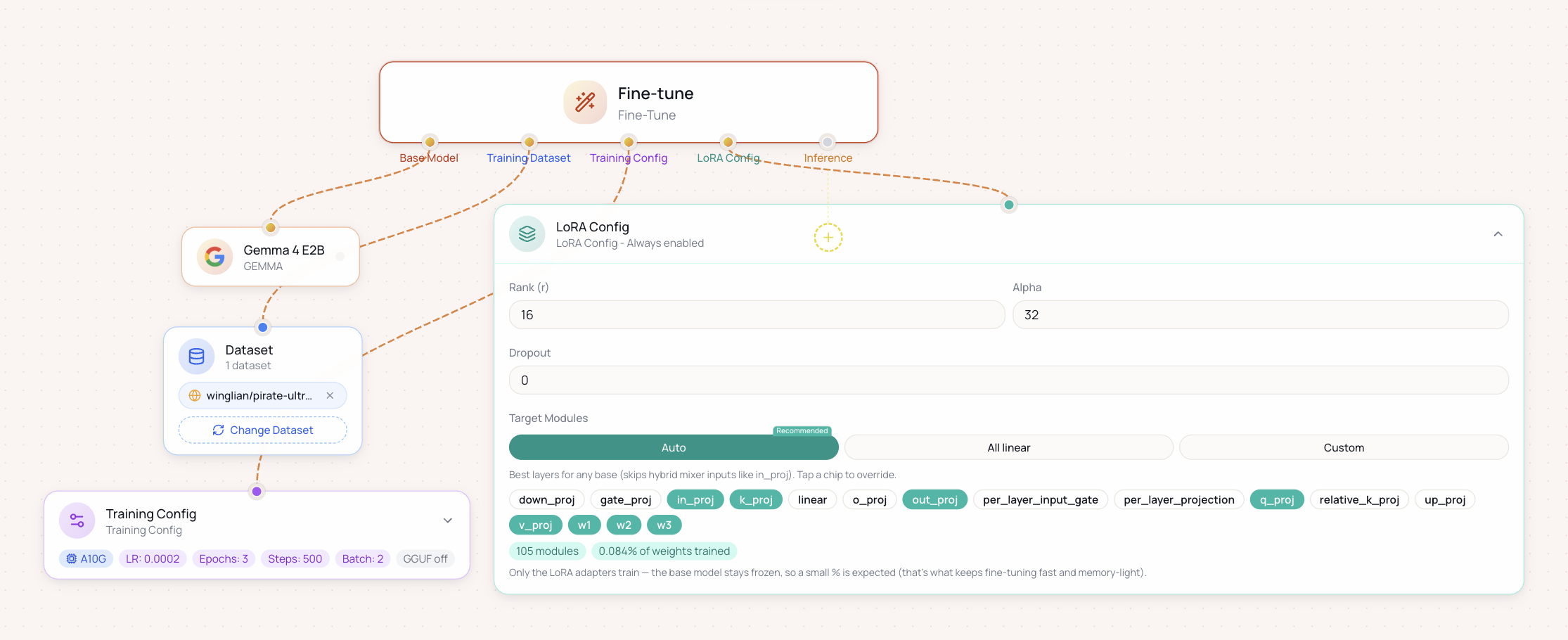
Target modules are the layers inside the model that the LoRA adapter attaches to. Ertas detects the modules that actually exist in your chosen base model and offers three ways to set them:
- Auto (recommended). The best set for any base, skipping hybrid mixer inputs like
in_proj. Use this unless you have a reason not to. - All linear. Adapt every linear layer. More capacity, larger adapter.
- Custom. Tap individual module chips to pick exactly which layers train. This is where detection matters: some architectures expose non-standard modules, and Ertas surfaces them so you can target them. Gemma 4 E2B, for example, exposes per-layer modules like
per_layer_input_gate,per_layer_projection, andrelative_k_projalongside the usual attention and MLP projections.
As you change the selection, Ertas shows a live count and the share of weights that will train (for example, "105 modules, 0.084% of weights trained"). Only the LoRA adapters train; the base stays frozen, so a small percentage is expected, and that is what keeps fine-tuning fast and memory-light.
Confirm and queue
When all four legs are green, the play button activates. Clicking it opens the Training Confirm dialog, which summarises:
- The base model and detected GPU tier.
- The datasets attached, with combined row count.
- The estimated step count and runtime.
- The estimated credit cost.
Pressing Start training queues the job and switches the canvas to Run mode. The Run panel slides in and your run appears at the top of the active list. See Training for what happens next.
Duplicating a recipe for parallel experiments
A common pattern is to test two hyperparameter settings side by side:
Build a base recipe
Configure a Fine-Tune module with all four legs.
Duplicate
Hover the module and click the purple Duplicate icon. Studio creates an identical recipe to the right, with its own child nodes.
Change one variable
Open the Training Config of the duplicate and change exactly one thing (for example, learning rate or LoRA rank).
Run both
Press play on both modules. They run in parallel, bounded by your credit balance rather than by a plan limit. See Parallel runs.
The Run panel labels each run with its module name, so name them clearly before duplicating.